Diagnosing GraphQL Latency with Traces and Request‑Scoped Batching

Thirty resolver calls can run together, or spend most of their time waiting for a dependency with limited capacity. A request count alone doesn't distinguish the two.
That matters when diagnosing a slow GraphQL operation. In the example here, request‑scoped batching reduces repository calls from 31 to three in both test conditions. In one condition, execution becomes substantially quicker. In the other, the median barely changes.
A trace helps explain why those two results differ. We also need to check that batching still returns the right data to the right person; fewer requests wouldn't be much of an improvement if they returned someone else's records.
One Programme, Thirty Screenings
The service has a fictional film programme containing thirty screenings across ten venues. Each venue appears three times. The client asks for the programme and each screening's venue:
query Programme {
  programme {
    id
    title
    venue {
      id
      name
    }
  }
}
Without batching, the programme resolver makes one repository call and each Screening.venue resolver makes another. That gives us 31 calls, including repeated lookups for the same ten venues. GraphQL.js's guide to the N+1 problem explains why independently composed resolvers need deliberate coordination for this kind of access.
The query doesn't reveal that implementation detail. The distinction between nodes and edges in Gatsby concerns the shape exposed by a schema; it doesn't tell us how many dependency calls a server will perform to produce it.
The local service, tests, and trace exports use GraphQL.js 17.0.1, DataLoader 2.2.3, and Node 22.23.4. The test client sends requests to a local HTTP endpoint, where GraphQL parses, validates, and executes them. Underneath that, I've used in‑process data and timers in place of a database. You can download the GraphQL batching experiment.
For the first condition, the programme read waits five milliseconds. Each venue call waits fifteen milliseconds, with at most three venue calls in service at once. A batch containing up to five venue keys pays one such delay. Those delays let us see what happens when calls have to queue. You'll need measurements from your own database to know how much each call actually costs.
Trace the Queue Separately from the Work
A resolver's duration includes time spent awaiting its dependency. If that dependency has a queue, calling the whole interval "database time" hides a useful distinction.
The example records a queue span before acquiring a service slot and a separate service span after acquiring it. Thirty sibling resolvers can start close together, but only three dependency calls can progress. The others wait for a slot.
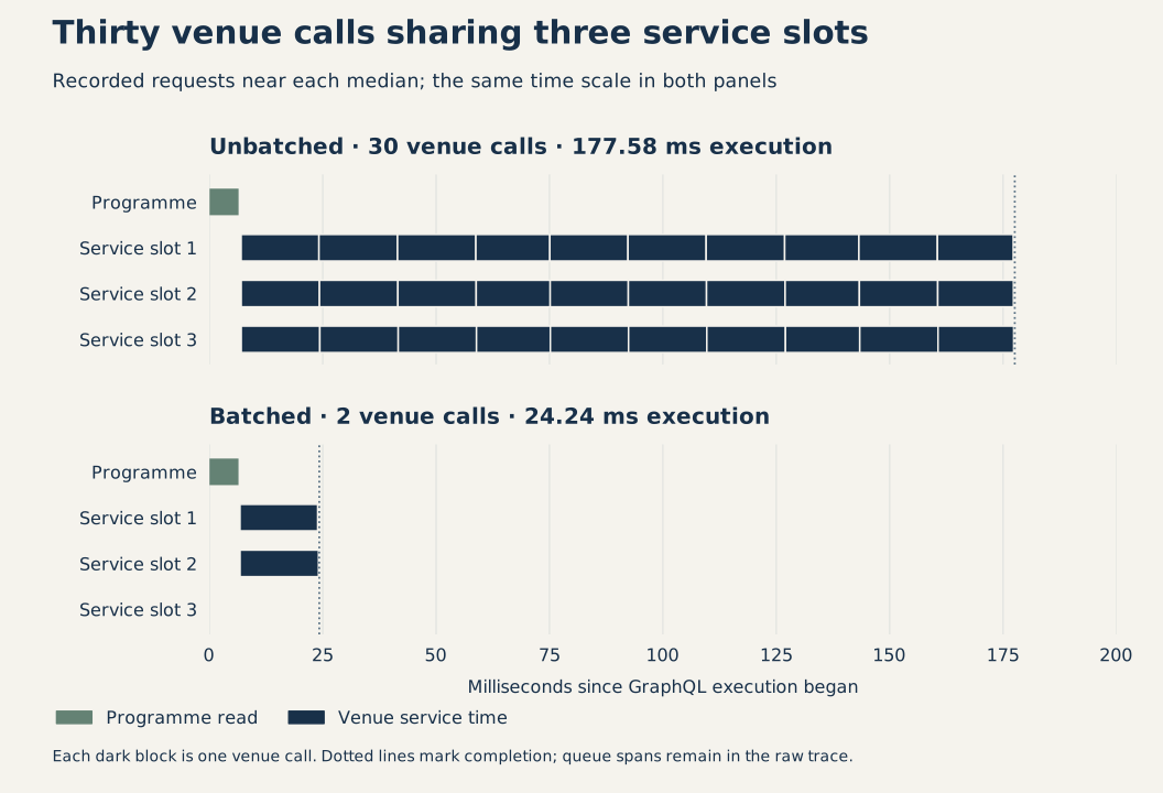
The figure uses individual recorded requests selected near their respective median execution times. Bars show actual synthetic service intervals, not configured timer lengths or an average trace. The full exports retain the queue spans as well.
In the unbatched measurements, the median of each request's longest queue wait was about 151.9 milliseconds. Batching reduced that figure to roughly 0.03 milliseconds. The individual service still waits for its timer; there are simply far fewer calls competing for the available slots.
Don't add every queue wait together and call the sum request latency. These intervals overlap. The same applies to parent and child spans: a resolver contains its awaited repository work, so summing both counts that time twice.
The trace records separate GraphQL parse, validation, execution, and response‑serialisation spans. Its surrounding processing span begins after credential resolution and request‑body parsing, and ends before writing the response. The client separately measures HTTP time through reading the response body. That gives us two different measurements: how long the selected server work takes, and how long the client waits for the response.
This follows the same principle as production observability: instrument the place where work actually happens. Here, manual wrappers record selected custom resolvers and repository work. They don't measure every scalar field, a federated gateway's query planner, or distributed network hops. GraphQL.js v17 also provides runtime tracing channels, but these particular traces don't use them.
Put the Loader Inside the Request
The example server looks up a fixed test credential to obtain a principal containing an actor, tenant, and permitted venue identifiers. It then creates a fresh context inside each execution:
const result = await trace.run('graphql.execute', root.id, async execution => {
  context = new Context(repository, principal, variant, trace, execution.id);
  return await execute({
    schema,
    document,
    contextValue: context,
    variableValues: input.variables,
    operationName: input.operationName,
    fieldResolver: resolver,
  });
});
Context constructs its own venue loader. The resolver calls context.venue(...), which either performs the individual lookup or uses that loader, depending on the variant being tested.
DataLoader doesn't recognise an HTTP request and reset itself automatically. Its cache belongs to the instance we create. Putting one instance at module scope would give it a much longer lifetime and could let one request reuse another request's result.
That becomes a correctness problem when identifiers overlap. Both festival tenants in the example have a venue called v6, with different names. Within one tenant, an editor can see all venues whilst a reader can see only five. The repository checks tenant and visibility on each actual read; the loader's request scope prevents cached results from bypassing those checks for another principal.
The fixed credentials are only there to exercise access checks; you'll need real authentication for a deployed service. The server derives the principal from its own map and ignores client tenant headers. A request‑scoped cache complements authorisation; it cannot supply the missing policy. The existing multi‑tenant application example develops that distinction further.
Keep Each Key in Its Original Position
The loader groups the ten unique venue identifiers into two batches of five. Repeated identifiers within the request reuse the same lookup. Here's the factory used by the example, including its trace links:
export function venueLoader(
  repository: Repository,
  principal: Principal,
  trace: Trace,
  executionId: string,
  contributors: Map<string, string[]>,
  cache = true,
): DataLoader<string, Venue | null> {
  return new DataLoader<string, Venue | null>(async keys => {
    const links = keys.flatMap(key => contributors.get(key) ?? []);
    for (const key of keys) contributors.delete(key);

    return trace.run('loader.batch', executionId, async batch => {
      const rows = await repository.venues(principal, keys, trace, batch.id);
      const byId = new Map(rows.map(row => [row.id, row]));

      return keys.map(key => repository.faults.perKey.has(key)
        ? new Error('Fixture venue error')
        : byId.get(key) ?? null);
    }, { keyCount: keys.length }, [...new Set(links)]);
  }, { maxBatchSize: 5, cache });
}
The faults.perKey branch is controlled test behaviour for investigating errors. The normal result comes from byId.
The repository deliberately reverses its returned rows and omits unavailable records. Returning that array directly would associate values with the wrong keys. Mapping over the original keys restores their positions, including null for a missing or inaccessible venue. The GraphQL field is nullable, so that absence doesn't erase the surrounding screening.
The DataLoader batch‑function contract requires one output position for each input position. The tests remove v2 and check that the first four screening venues are v1, null, v3, and v4. They also disable caching and verify repeated keys remain repeated output positions. Deduplicating the repository lookup mustn't shorten the result array.
maxBatchSize bounds the number of keys in one batch. It doesn't impose the repository's concurrency limit, and it doesn't promise that every lookup throughout an operation joins one batch. This query's sibling lookups arrive together; later dependent work can create another batch.
A batch also has several callers. The trace therefore places it beneath execution and links it to its contributing resolver spans, rather than assigning an arbitrary resolver as its sole parent. Each five‑key batch in this query links fifteen resolver invocations, because each venue appears three times.
Repeat the Measurement with a Different Bottleneck
The second condition makes the programme read slow: its configured delay is 120 milliseconds. Venue calls still have a fifteen‑millisecond delay, but there is no configured concurrency cap. The unbatched calls can overlap once the programme arrives.
Both conditions use two excluded warmups followed by ten measured requests per variant, alternating variant order. All forty measured responses contain identical data and have the same 2,412‑byte JSON body. Traces stay on the server, identified by a response header, so extra spans don't inflate the measured response payload.
| Condition | Variant | Repository calls | Median execution | Observed execution range |
|---|---|---|---|---|
| Three venue service slots | Unbatched | 31 | 176.91 ms | 173.73–181.88 ms |
| Three venue service slots | Batched | 3 | 24.24 ms | 22.60–24.94 ms |
| Slow programme, uncapped venue calls | Unbatched | 31 | 140.89 ms | 139.35–141.62 ms |
| Slow programme, uncapped venue calls | Batched | 3 | 140.61 ms | 137.95–142.06 ms |
The slow‑programme condition retains the same reduction in calls, but almost none of the earlier latency benefit. Its programme span takes around 122 milliseconds in both variants. Batching hasn't changed that dependency.
The corresponding HTTP medians were 181.00 and 26.83 milliseconds for the queued condition, then 144.63 and 144.31 milliseconds for the slow‑programme condition. Those small differences in the latter pair don't support a useful speed claim.
These are local observations on an Apple M2 with 24 GiB of memory, using one Node process and sequential test requests. Timer scheduling and shared‑host noise affect the timings; the raw results retain every sample. They aren't production percentiles, throughput measurements, or evidence that a real five‑key database query costs the same as one single‑key query.
Exercise the Cache After the Happy Path
The eleven groups of tests exercise the loader directly and through HTTP requests. Here are the cases they cover:
| Case | What is verified |
|---|---|
| Concurrent requests with overlapping IDs | Distinct loader scopes preserve both tenant and actor visibility |
| A client sends another tenant's header | The server‑derived principal still controls access |
| Rows arrive reversed or a venue is absent | Results preserve the requested order and missing positions |
| One key returns an error | That error is cached until explicitly cleared |
| The entire batch rejects | Later loads retry instead of reusing the failed batch |
| Caching is disabled | Duplicate keys still receive separate output positions |
| A venue is renamed | Same‑request rereads and a subsequent request see the new value |
The mutation deliberately reads before writing, so the loader already contains the old value. After the authorised repository update, it clears that key before reading again:
const before = await context.venue(id, span);
await context.repository.rename(context, id, args.name as string, span);
context.loader.clear(id);
const after = await context.venue(id, span);
return { before, after };
The editor receives the old and new names as expected. A reader's attempted write is rejected even for a venue they may view, and the stored value remains unchanged.
To show what goes wrong, a separate test deliberately shares a loader. After caching North's v6, it changes the active principal to South and receives North's cached value. It then changes to North's restricted reader and exposes the same hidden venue. The HTTP service always creates a loader for each request. Once you've seen the shared loader return another tenant's venue, it's easier to see why its lifetime matters.
Use the Remaining Trace to Choose the Next Change
In the queued condition, reducing repeated venue work removes substantial waiting. In the slow‑programme condition, the next investigation belongs in the programme dependency. Adding another cache layer without understanding that read would obscure the question.
A production investigation still needs the actual dependency's query plan, indexes, network behaviour, and load constraints. This example doesn't measure those things, or include a gateway, query‑cost limits, or a distributed cache. What we can see is where batching removes waiting, where it makes little difference, and whether the results and access checks still behave correctly.